ReflexFlow: Rethinking Learning Objective for Exposure Bias Alleviation in Flow Matching

Despite tremendous recent progress, Flow Matching methods still suffer from exposure bias due to discrepancies in training and inference. This paper investigates the root causes of exposure bias in Flow Matching, including: (1) the model lacks generalization to biased inputs during training, and (2) insufficient low-frequency content captured during early denoising, leading to accumulated bias. Based on these insights, we propose ReflexFlow, a simple and effective reflexive refinement of the Flow Matching learning objective that dynamically corrects exposure bias. ReflexFlow consists of two components: (1) Anti-Drift Rectification (ADR), which reflexively adjusts prediction targets for biased inputs utilizing a redesigned loss under training-time scheduled sampling; and (2) Frequency Compensation (FC), which reflects on missing low-frequency components and compensates them by reweighting the loss using exposure bias. ReflexFlow is model-agnostic, compatible with all Flow Matching frameworks, and improves generation quality across datasets. Experiments on CIFAR-10, CelebA-64, and ImageNet-256 show that ReflexFlow outperforms prior approaches in mitigating exposure bias, achieving a 35.65% reduction in FID on CelebA-64.

Mainstream training paradigms aim to mitigate bias during training by simulating the inference process. For instance, IP injects perturbations into real data, and methods like MDSS/SDSS align the training target with anticipated inference dynamics. Despite improving robustness to biased inputs, these methods do not fundamentally eliminate the inherent bias induced by the training-inference mismatch.

1. The Limitation of Standard Flow Matching

By analyzing the reverse denoising process (reparameterized by time $\tau = 1 - t$), we formally derive the bound for the expected final sampling error $\mathbb{E}\|\mathbf{e}_{\tau_k}\|$ under the standard FM objective:

The error decomposes into the Integrated Ground Truth Velocity Residual and the Integrated Exposure Bias. Standard FM training only minimizes the first term ($\mathbb{E}\|\mathbf{r}_\tau\|^2$), leaving the exposure bias term unaddressed. This allows bias to accumulate linearly, contributing significantly to the final sampling error.

2. Theoretical Guarantee of ADR

To address this, we propose Anti-Drift Rectification (ADR). We prove that the error bound under ADR is governed by a fundamentally different mechanism:

Here, $\pmb{\phi}_\tau$ represents the ADR residual. Crucially, the exposure bias term is algebraically cancelled, and the remaining Path-Geometry Constant is independent of model errors. Thus, the final sampling error is determined purely by the Integrated ADR Residual, which ADR explicitly minimizes. This turns uncontrolled exposure bias into a learnable quantity.

3. Reliability and Effectiveness

Furthermore, we prove that the ADR bound is order-equivalent to the FM bound ($B_{\mathrm{ADR}} \le C_1 B_{\mathrm{FM}} + C_2$). This ensures that $B_{\mathrm{ADR}}$ provides an error estimate with reliability comparable to $B_{\mathrm{FM}}$, while offering complete control over exposure bias that standard FM lacks.

Beyond prediction drift, our investigation uncovers a critical spectral imbalance in standard Flow Matching. [cite_start]Frequency analysis of early denoising predictions reveals a significant deficiency: the model consistently fails to capture sufficient low-frequency components in its initial outputs[cite: 68]. [cite_start]This deficiency leads to substantial error propagation during the crucial early stages of generation[cite: 69].

1. Quantifying Frequency Deficiency

To rigorously analyze this, we introduce two metrics:

[cite_start]
• $R_{\text{LFDV}}$ (Low-Frequency Dominant Ratio on Velocity): Measures the ratio of low- to high-frequency energy in the model’s predictions, capturing how much low-frequency content the model produces at each step[cite: 70].
[cite_start]
• $R_{\text{LFDL}}$ (Low-Frequency Dominant Ratio on Loss): Measures the relative emphasis the learning objective places on low- versus high-frequency regions of the target velocity[cite: 71].

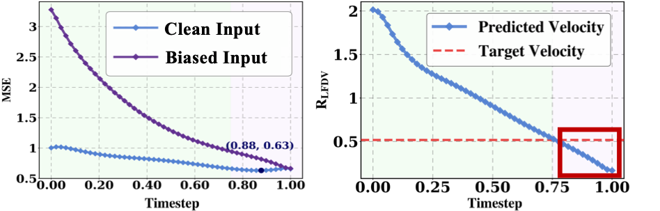
Figure 2: Quantitative Analysis of Exposure Bias in Flow Matching. Left: Mean squared error (MSE) comparison showing exposure bias significantly increases error under biased inputs. Right: Frequency distribution analysis. [cite_start]Early denoising predictions (purple background) consistently lack low-frequency components (red box), while later steps (green background) show a high-frequency deficiency[cite: 38, 39, 40].

As highlighted in Figure 2 (right), the low-frequency energy in FM predictions remains consistently below the ground truth during early denoising. [cite_start]Since low-frequency components encode critical structural information, this insufficiency significantly degrades overall generation quality[cite: 73, 74].

2. The Complementary Nature of Exposure Bias

[cite_start]Interestingly, our analysis reveals a unique property of exposure bias: it exhibits a complementary, low-frequency-dominated characteristic at early timesteps[cite: 75].

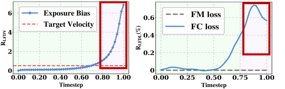
Figure 3: Exposure Bias and Frequency Compensation. Left: Evolution of exposure bias frequency distribution. Early timesteps are dominated by low-frequency components (red box). [cite_start]Right: The proposed exposure-bias-reweighted loss effectively emphasizes these missing low-frequency components at early timesteps compared to the original objective[cite: 57, 58].

3. Visualizing the Compensation Mechanism

To verify this, we visualize the spatial distribution of exposure bias. [cite_start]The heatmaps confirm that exposure bias is strongly concentrated in low-frequency regions during high-frequency timesteps (HFT), aligning closely with the low-pass filtered ground truth[cite: 243].

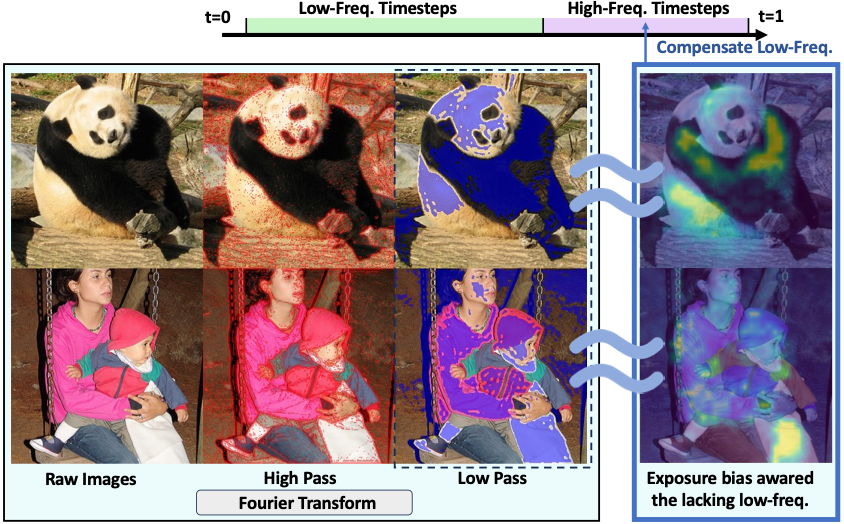
Figure 4: Visualization of Dominant Frequency Regions. Comparison of original images (left) with exposure bias heatmaps (right) at HFT. [cite_start]The exposure bias heatmaps (right) correspond closely to the low-frequency components (blue mask) of the ground truth, revealing that exposure bias naturally highlights the missing structural information[cite: 260, 261].

Based on these insights, Frequency Compensation (FC) leverages exposure bias as a reweighting signal. [cite_start]By effectively emphasizing the absent low-frequency information in the loss function, FC mitigates exposure bias at its root source[cite: 79].

1. Anti-Drift Rectification (ADR)

Our theoretical analysis reveals that the original Flow Matching objective is blind to exposure bias. To address this, we must introduce a training signal that explicitly constrains the drift. However, simply minimizing exposure bias is ineffective as it encourages the model to follow the drifted path. Instead, we propose to align the model’s output velocity at the drifted state back toward the target endpoint.

We define the Anti-Drift Velocity Target as:

Considering the magnitude discrepancy between predicted and anti-drift velocities, we focus on aligning their directions. The rectification loss is defined as:

2. Frequency Compensation (FC)

[cite_start]Motivated by the observation that exposure bias naturally highlights missing low-frequency content (as shown in our motivation analysis), we design a negative-feedback weight mask to reweight the original loss[cite: 1, 2].

The spatial weight map is calculated based on the exposure bias $\pmb{\delta}_{\text{exp},t}$:

We then use this weight to refine the original Flow Matching objective, adaptively emphasizing the missing frequency components at each timestep:

3. ReflexFlow Framework

ADR learns to correct the exposure bias that has already occurred during inference, while FC mitigates exposure bias at its source during training. These two mechanisms complement each other.

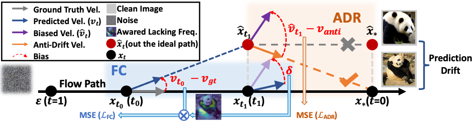
Figure: Overview of ReflexFlow. (a) Anti-Drift Rectification constructs a new learning objective to guide the model from the drifted distribution back to the true data distribution. (b) Frequency Compensation uses exposure bias as a negative-feedback signal to reweight the original objective, mitigating low-frequency deficiency.

We integrate them into a unified framework, ReflexFlow. The final learning objective combines both mechanisms:

where $\beta_1$ and $\beta_2$ are weighting coefficients. ReflexFlow thus provides a simple yet effective solution to exposure bias, enhancing both prediction accuracy and generation quality.

1. Quantitative Results

We reproduce key experiments to ensure fair comparison under identical training environments. Our main findings are summarized as follows:

• ReflexFlow consistently improves SiT: Reducing FID by 9.01%/11.16% on ImageNet-256 (w/o and w/ cfg=1.5), 9.56%/18.49% on CIFAR-10, and 14.88%/35.65% for unconditional CIFAR-10 and CelebA-64.
• ADR surpasses MDSS and SDSS: Unlike SDSS which uses ground-truth targets, ADR learns a reconstructed anti-drift target, demonstrating the benefit of dynamic target rectification.
• Complementary Benefits: Both ADR and FC individually improve generation, and their combination in ReflexFlow achieves the best performance.
• Superiority over Prior Methods: While prior methods rely on input perturbation (IP) or post-inference alignment, ReflexFlow directly corrects prediction drift and compensates missing frequency components at the source.

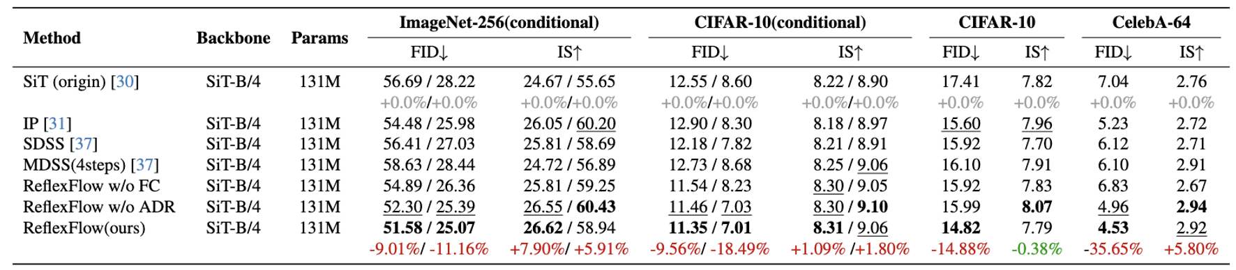
Table 1: Quantitative comparison of different methods across different datasets.
Class-conditional generation on ImageNet-256 and CIFAR-10, and unconditional generation on CIFAR-10 and CelebA-64. All entries are reported using 50-NFE samplings. Red highlights improvements by our method, green indicates deficits compared to the baseline.

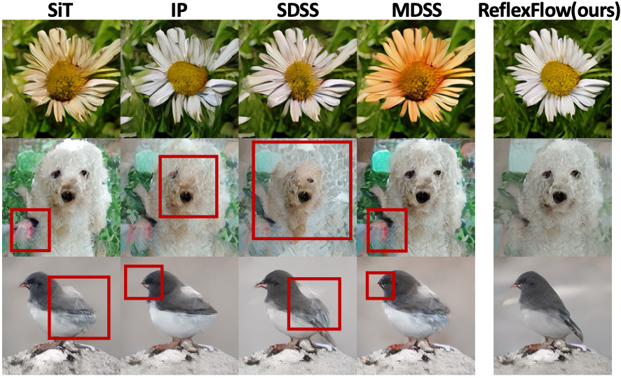
2. Qualitative Results

All methods use the same random seed and 50-NFE inference for fair comparison. As shown in the figure below, baseline methods exhibit clear visual artifacts:

• Blurred Boundaries: The second and fourth rows show blurred object–background boundaries.
• Structural Distortions: The first and third rows display structural distortions and missing details.

These issues arise from exposure bias accumulating during High-Frequency Timesteps (HFT), causing confusion between the primary object and surrounding context. In contrast, ReflexFlow generates images with more coherent structures and consistent textures by suppressing prediction drift and compensating missing frequency components.

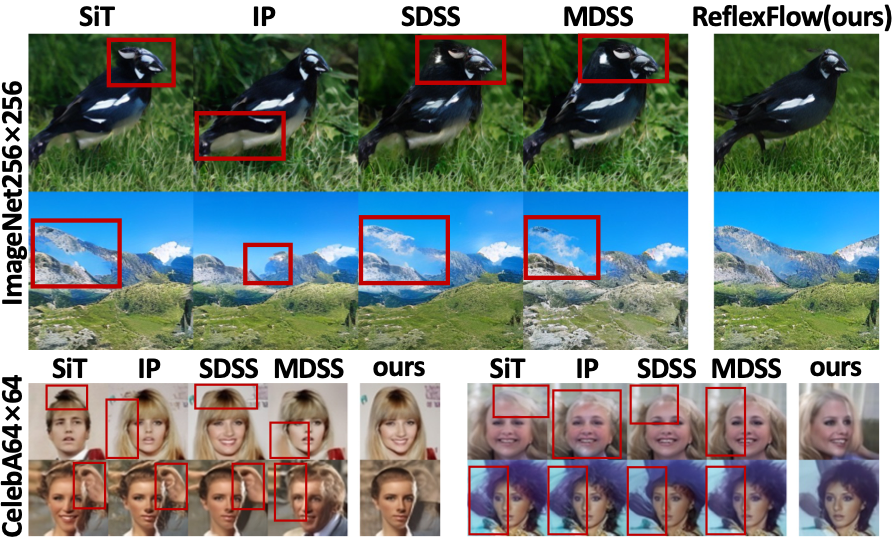
Figure 6: Qualitative Comparison.
ReflexFlow produces the most realistic samples on ImageNet-256 and CelebA-64, clearly outperforming baselines which exhibit blurriness or distorted details (highlighted with red boxes).

1. Superior Mitigation of Exposure Bias

ReflexFlow outperforms prior methods in mitigating exposure bias. [cite_start]We quantify this by computing the relative MSE changes (with vanilla SiT as the baseline) between predicted and ground-truth velocities during inference[cite: 163]. [cite_start]As shown in the figure below, ReflexFlow achieves the lowest bias across all timesteps, demonstrating its superior capability to mitigate exposure bias[cite: 164].

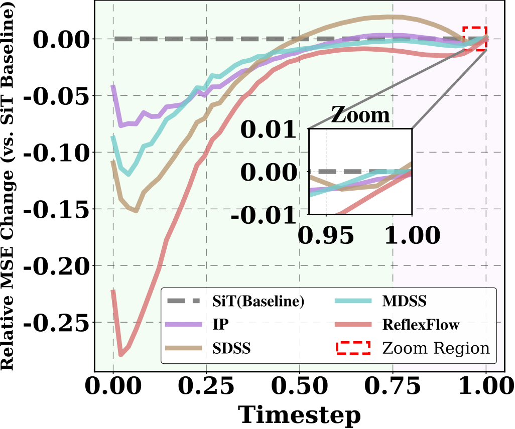
Figure: Quantitative analysis of exposure bias over timesteps. We measure the MSE between predicted and ground-truth velocities for all methods relative to the SiT baseline. [cite_start]ReflexFlow consistently achieves the largest reduction[cite: 147].

2. Scalability of ReflexFlow

ReflexFlow exhibits strong scalability in generative quality. [cite_start]As shown in the table below, our method consistently outperforms original SiT models across different model scales[cite: 167]. [cite_start]Given the emergence of scaling laws in AIGC, ReflexFlow is well-positioned to leverage these trends for scalable, high-fidelity generation[cite: 168].

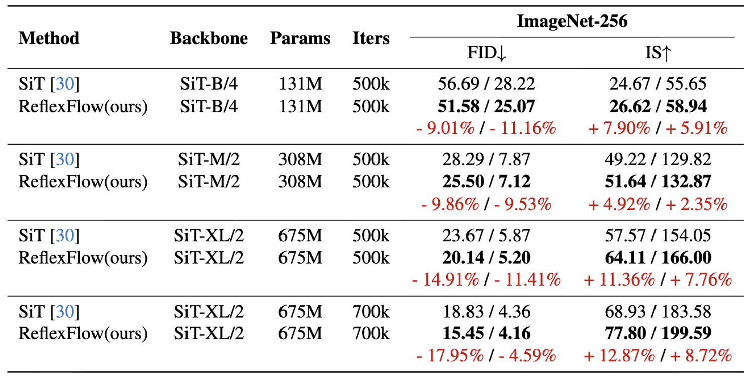
Table: Scalability of ReflexFlow on ImageNet-256. 50-NFE generation without/with cfg=1.5. [cite_start]Models are trained from scratch[cite: 145].

3. Robustness under Extended Inference

Potential prediction bias accumulates over time. [cite_start]Increasing inference steps often amplifies exposure bias and degrades generation quality[cite: 170]. [cite_start]To assess this, we evaluated methods under various step settings (30, 50, 100, 250, 500)[cite: 171]. [cite_start]ReflexFlow consistently achieves the lowest FID and highest IS, maintaining stable performance as sampling steps increase, whereas baselines degrade noticeably[cite: 172].

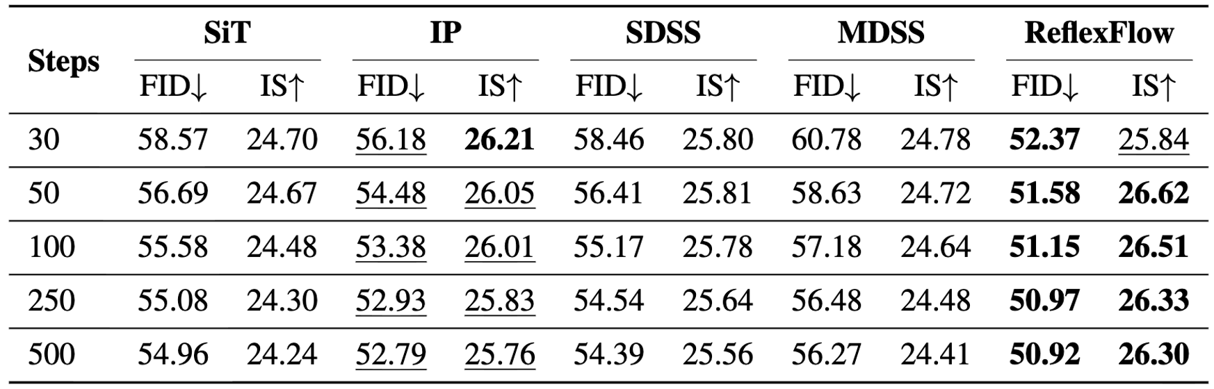
Table: The effect of multi-NFE sampling on ImageNet-256. Entries are reported without cfg. [cite_start]ReflexFlow remains strong even at 500 steps[cite: 150].